Session 0
Content
- Philosophy behind these instructional materials
- Why R?
- Introduction to R
- Installing R, RStudio, and tidyverse
- Getting settled in RStudio
Philosophy
I have never taken a course or workshop in using R. I’ve read a lot of books on how to program with R. To be honest, I’m not sure how much they helped. I learned R by taking a single script that I wrote to create a scatter plot and modifying it or “hacking it” to get it to do what I wanted. If I ran into a problem, I would either google the error message or the question I was trying to answer. As I asked around, I learned that most people learned R by hacking their way to success along with a lot of practice. That is the underlying philosophy of this series of lessons. Most programming books slowly build to something useful with silly examples along the way. The first code you will write in Session 1 will be the basis of every other piece of code we write in these tutorials. We will start with working code for a plot that could be published and hack it until we have a plot showing which taxa are associated with health or disease.
I suspect that you will understand the first chunk of code we write. We will strive for readable code that is easy to understand. That being said, just because you suspect that the geom_point function will add points to a plot, doesn’t mean that you know how to use geom_point or that you would know how to make a bar chart. Calmly accept your ignorance and know that all will be explained eventually. Learning experts have found that we do not learn best by taking on a topic and beating it to death until we’ve mastered it. Rather, we learn best when we learn something partially, move on to something else that we also learn partially, but can fold in the previous knowledge to help us improve our partial knowledge of the earlier topic. It’s kind of like taking steps forward in a dark room only to get to the end and see that you knew the path all the way along. This is the approach that we will be taking with these lessons. My goal is not to provide a reference on R or to necessarily document every nook and cranny of the language and its myriad packages. I will empower you to do that.
The final philosophical point I will make is that I believe it is important to eat your own dog food as an educator. Everything I teach, is how I want to code and how I want those that work for me to code. There is definitely always room for improvement, but be confident that I’m not trying to sell you on something that I do not use myself. That being said, although I don’t claim that the plots we’ll make are works of aRt, I do think that they’re pretty close to being publication quality. Why make a crappy plot, when you could make a good one that puts your work in the best possible light?
If you notice a bug, something that is unclear, have an idea for a better approach, or want to see something added, please file an issue or, even better, a pull request at the project’s GitHub repository.
Why R
If you’re looking for some big “pound your chest” explanation for why you should learn R, then you’re looking in the wrong place. I know R. That’s why I teach R. Why did I learn R? There were people around me that new R and I knew I could depend on them to help me learn R if I ran into any problems. Less important than which language you should learn is that you learn A language. Any language, really.
The way I see it there are several credible languages if you are a scientist: R, Python, C/C++, Java. R and Python are “high level” languages that have a lot of built in goodies to make your life easy. As you’ll see, it’s pretty easy to build a graph or to calculate a mean in R (and python). These languages are engineered to make it easier on the programmer than the person running the code. In contrast, C/C++ and Java are not as easy to program, but are far more efficient and run blazing fast. You’ll hear about others like Julia, Ruby, or Perl. These aren’t quite mainstream for biologists or aren’t fully developed yet or are past their sell by date. Unless you have needs for high performance, I’d probably stay away from C/C++ and Java isn’t really all that high performance. If you need the speed of C++ you can write C++ in R.
This leaves you to chose between R and Python. You can google “Should I learn R or Python” and you’ll get screed after screed telling you why one language is the best. Do not read these. They’re next to worthless and smack of all sorts of machismo. I block accounts on Twitter that go off on R vs. Python screeds. I know R’s warts and I know that Python could possibly cure these warts. But I also know that Python has its own warts. Rather than carry the cognitive baggage of learning both, I do what I need in R. At least a few times a year I tell myself I should learn Python to know it, but when it comes to doing it, I’m just not sold. To be honest, to really appreciate the differences between the languages you probably need a fair bit more experience than someone that is reading this. Note that someone else could/should easily rewrite this paragraph switching R and Python.
But really! What should you learn? Depends. What does your research group use? What do your collaborators use? What do the people around you use? If you have a problem, who are you going to get help from? For me, the answers to these questions were generally: R. Again, it’s more important that you learn your first language than which language you learn. Master your first language and then start noodling with others. I always cringe when I see someone encouraging a novice to learn other languages. It can only sow confusion and frustration. Since you’re here, I suspect someone has encouraged you to learn R or that your local community has some R chops. Welcome! I want to challenge you to not just use your community to help you, but to also nourish your community to help it grow.
What you need to do these tutorials…
Before starting the tutorials, you will need to install a few tools:
- R: These materials have been tested using R version 4.0.3 (2020-10-10)
- RStudio: These materials have been tested using RStudio version 1.4.1103
- Raw data files: Download using the “Source Code (zip)” link. This will download a directory called
generalR_data-0.2where the “-0.2” is the version number. Make sure the directory is uncompressed and remove the “-0.2” so that you now have a directory called generalR_data. This is super important!
Later, we’ll install the tidyverse package from within RStudio. Go ahead and click on the links for R and RStudio to install them on your computer. You need both.
Customizing RStudio
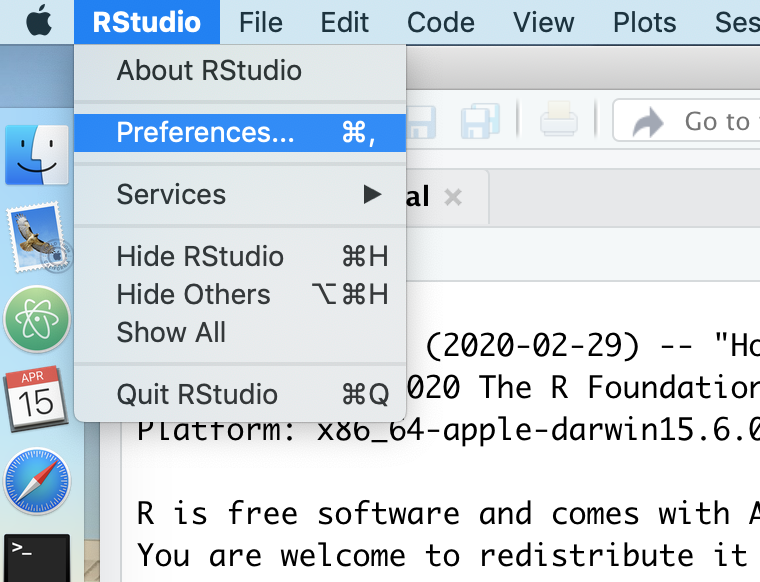
There are many ways to customize RStudio. You can find the options by going to the Preferences window. If you are using windows you can get to the Preferences window by going Tools->Global Options. Here is a screenshot of how to do it for Mac OS X. The method should be pretty similar for people working on a Windows computer.
In the first tab, “General”, you should have something like this.
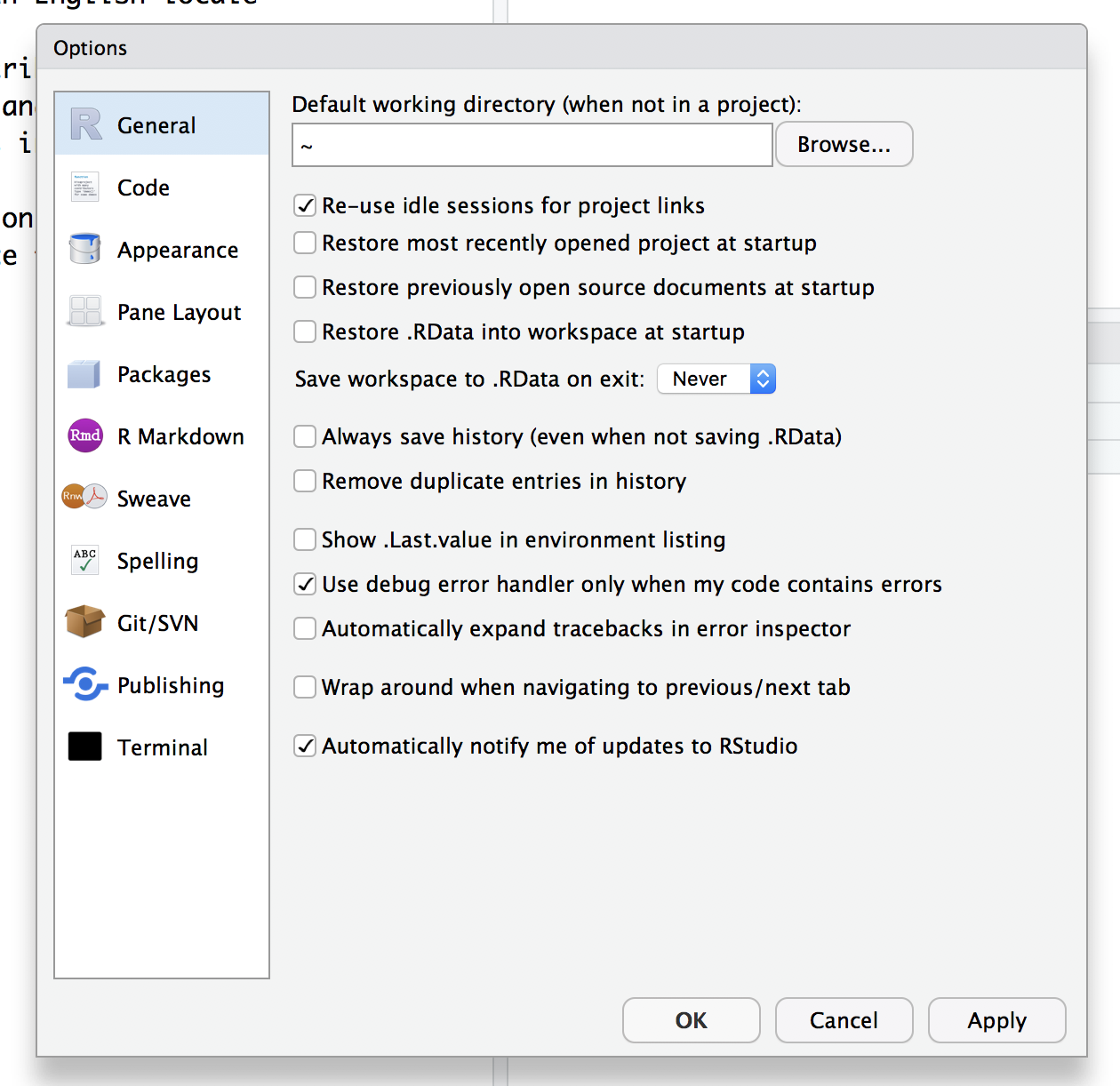
You don’t want any of the boxes to be checked except to be notified of RStudio updates, these are especially problematic:
- Restore .RData into workspace at startup
- Save workspace to .RData on exit (toggle should say “Never”)
- Always save history
Once you’ve got everything checked/unchecked the way you want it, go ahead and click “Apply” and then “OK”
Oversized calculator
On the left side there is a tab for console. This is where we will be entering most of our commands. Go ahead and type 2+2 at the > prompt (don’t type the >, that’s the prompt)
> 2+2
## [1] 4
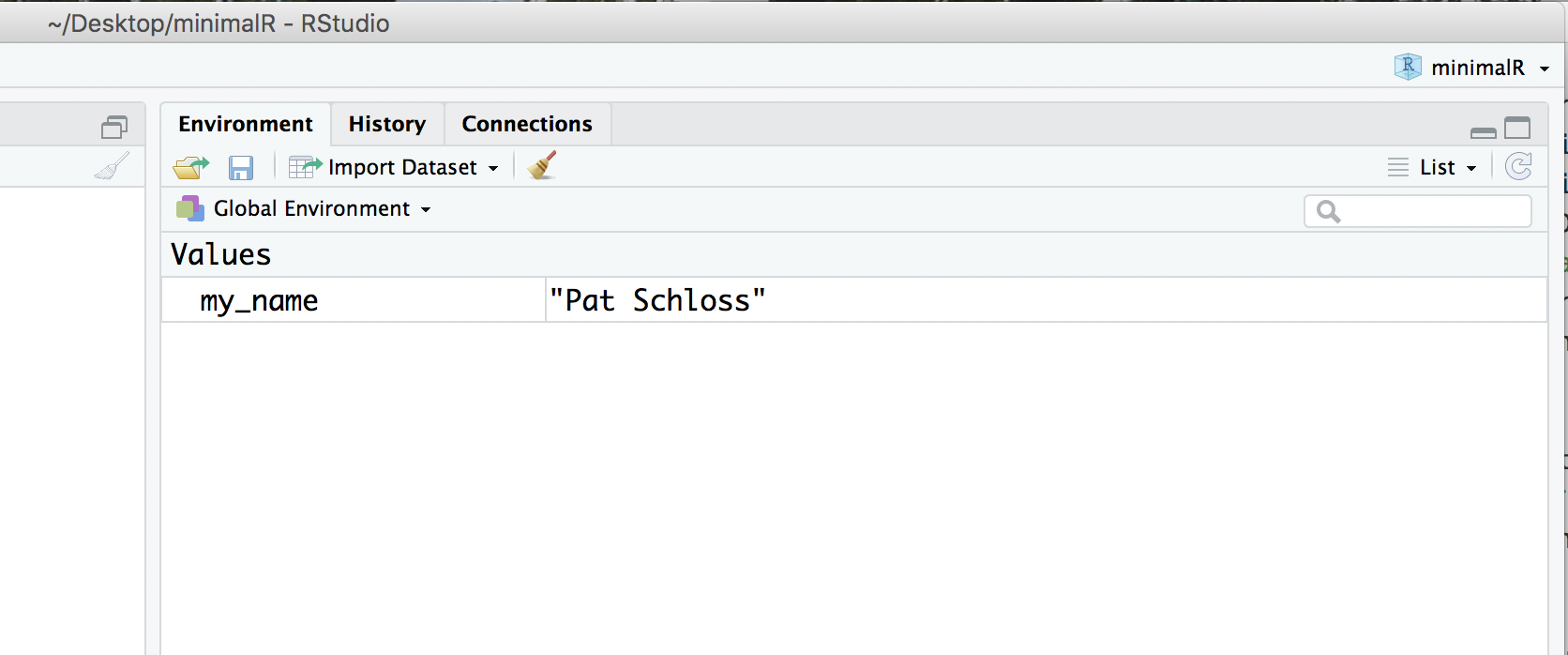
Now type the following at the prompt (feel free to use your own name)
> my_name <- "Pat Schloss"
Now look in the upper right panel. In the “Environment” tab you’ll see that there’s a new variable - my_name and the value you just assigned it. We’ll talk more about variables later, but for now, know that you can see the variables you’ve defined in this pane.
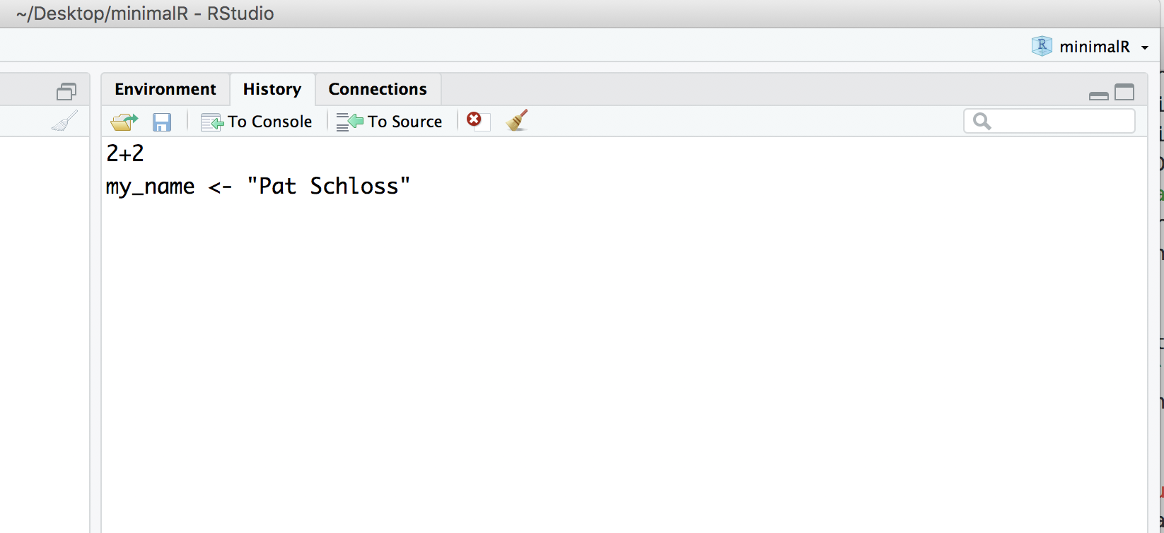
Go ahead and click on the “History” tab. There you’ll see the last two commands we’ve entered.
Installing packages
There’s a lot of functionality built into R. The beauty of it being an open source resource is that anyone can add to it to expand it’s functionality or to improve how you work with the existing functionality. This is done through packages. Some day, you might make your own package! We will use several R packages throughout our Code Clubs. The one we’ll use the most is called tidyverse. We’ll be talking a lot about this package as we go along. But for now, we need to install this package. In the lower right panel of RStudio, select the “Package” tab. You’ll get something that looks like this:
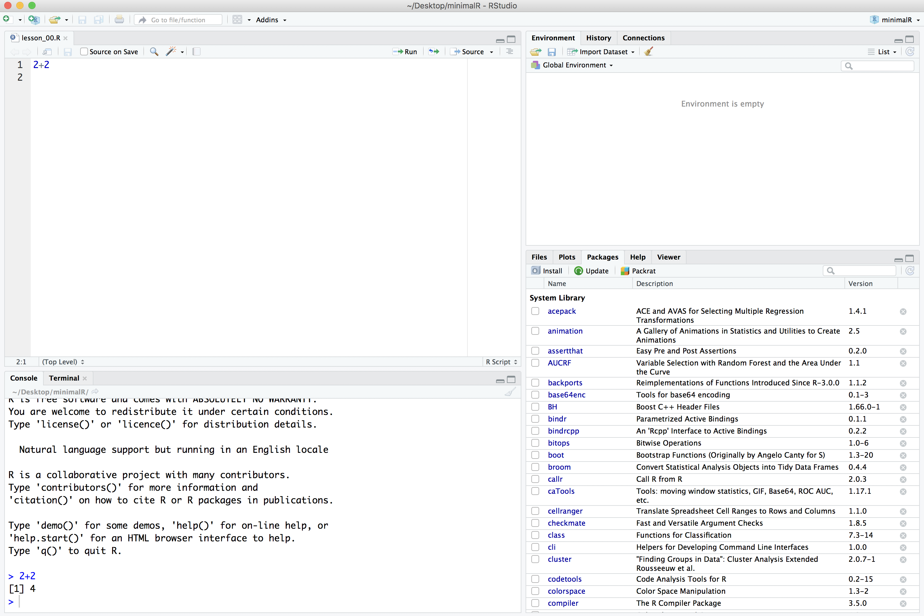
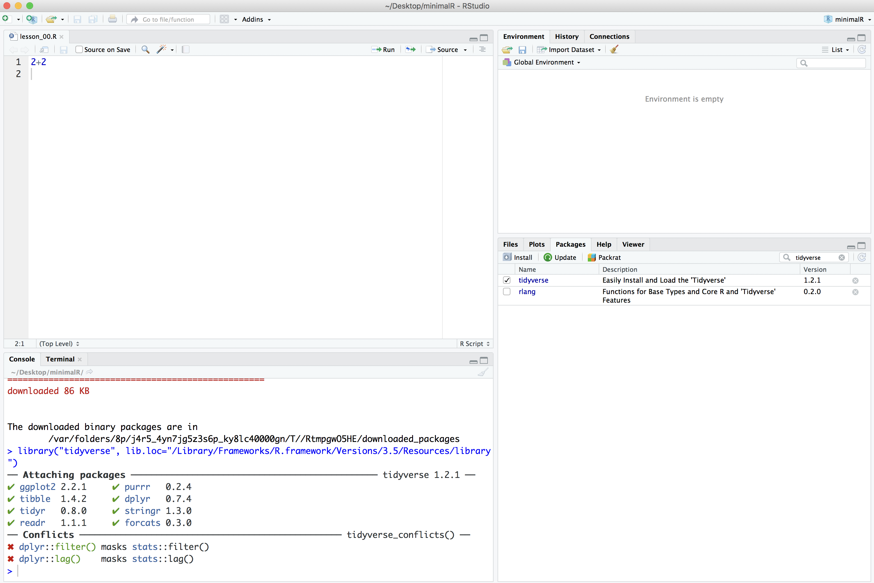
In the search window, type in “tidyverse” (without the quotes). If it isn’t already installed, you won’t see it. If it is installed, it will be listed. The package isn’t installed on my computer.
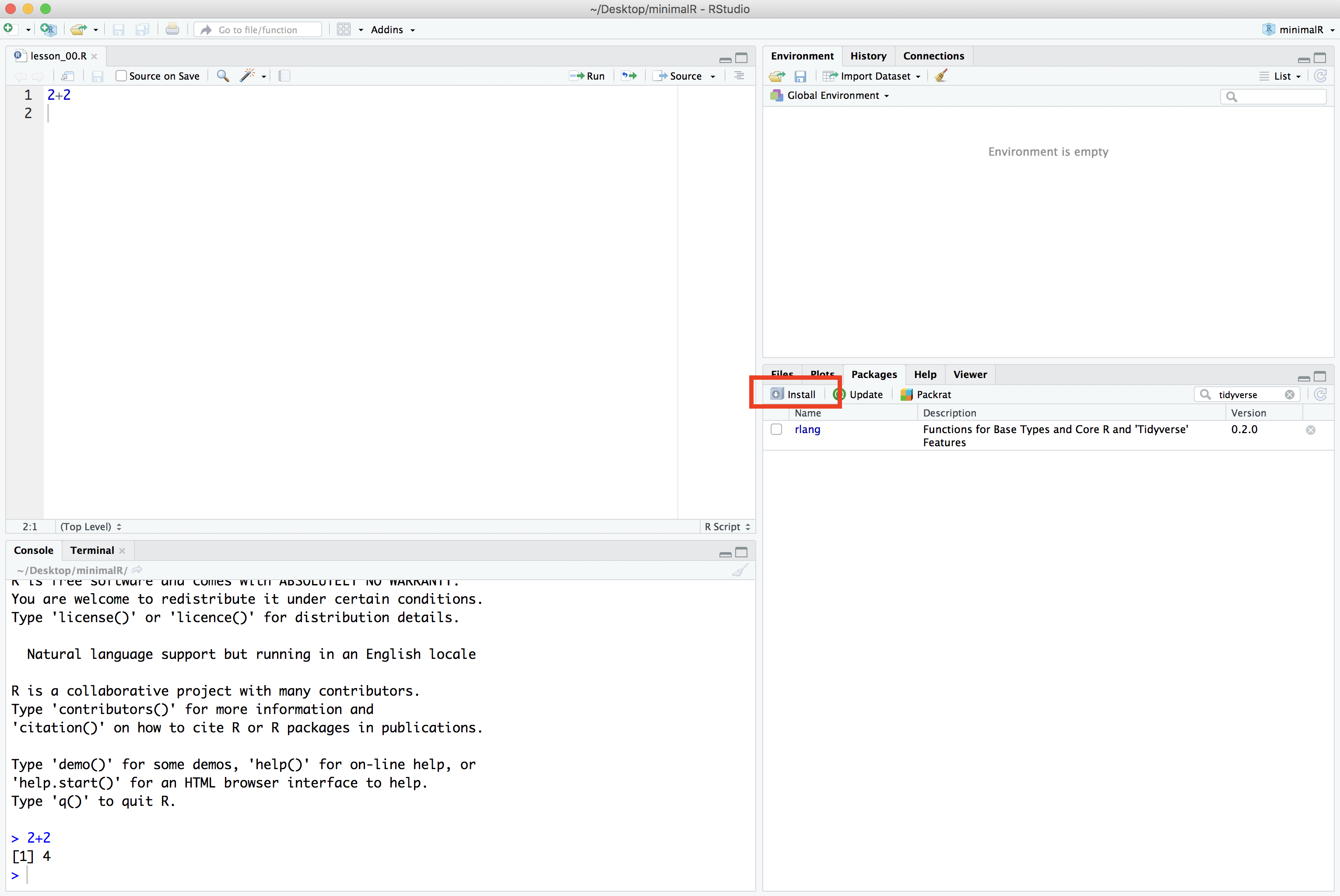
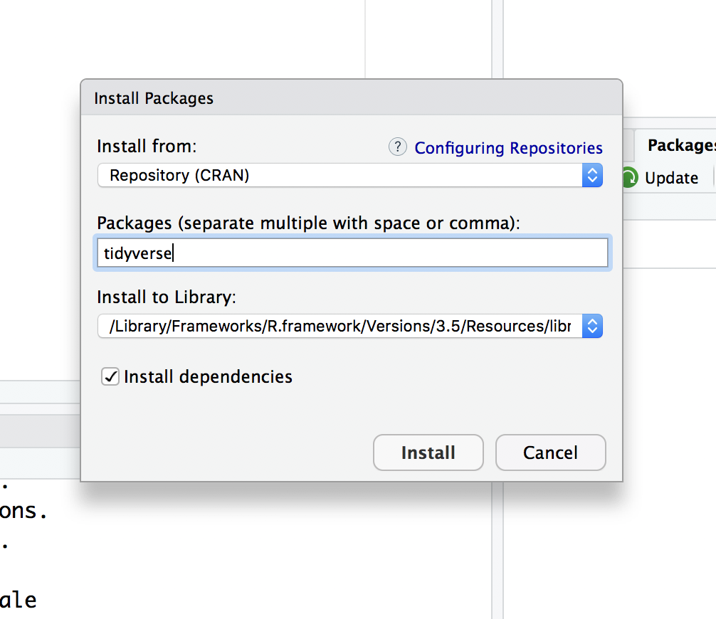
If it isn’t installed on your computer either, go ahead and click the Install button and type “tidyverse” into the “Packages” window:
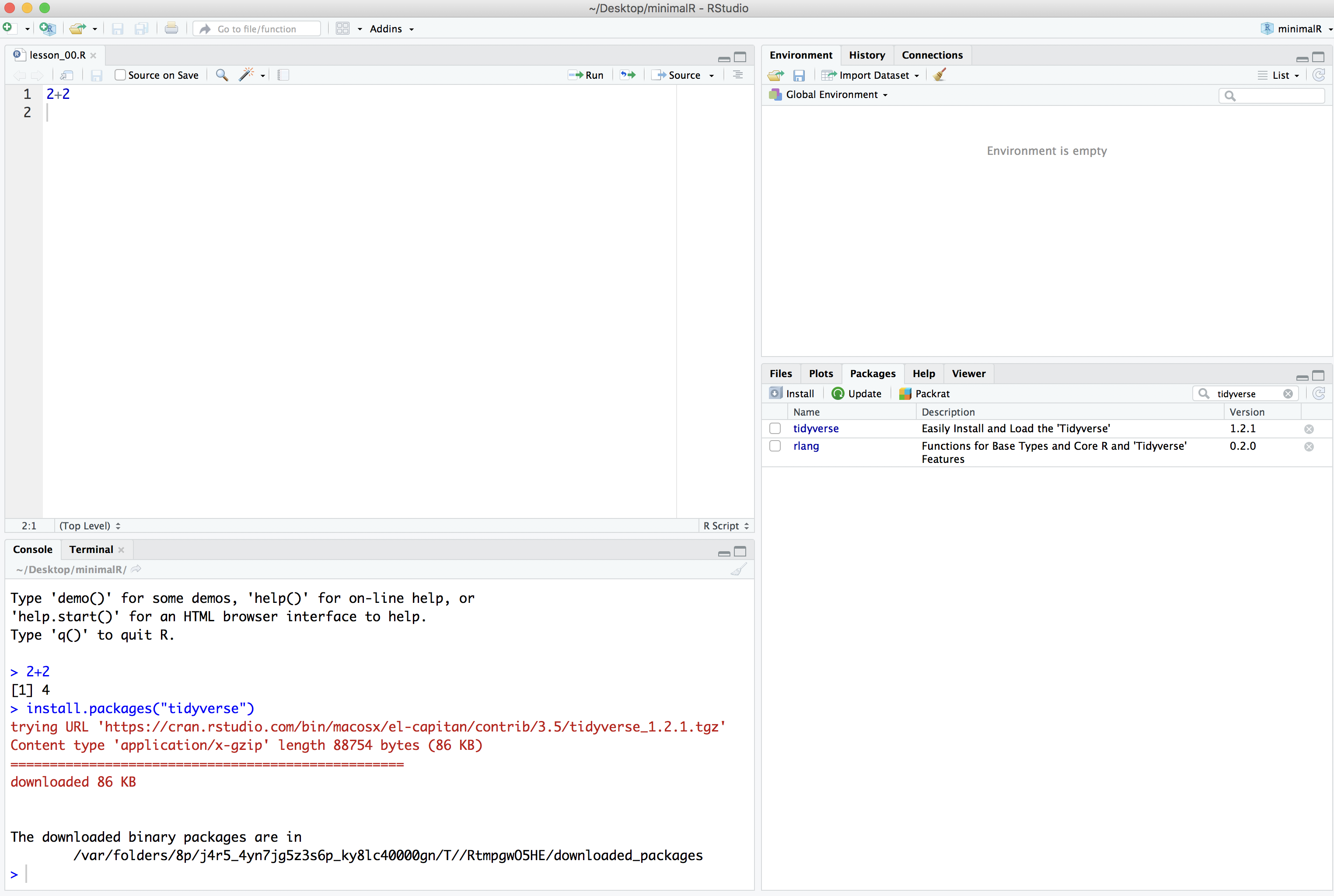
Once you press the “Install” button, the dialog will close and RStudio will install the package. You’ll notice a couple things have happened. In the Packages tab in the lower right panel, you now see the “tidyverse” package is there. You’ll also notice that in the lower left corner that R ran the command install.packages("tidyverse").
Finally, to make all of the tidyverse goodness available as we go through the tutorials, you can either click the small square next to “tidyverse” in the “Packages” tab or you can run library(tidyverse) in the console tab in the lower left panel of RStudio.
Some things may happen…
- While loading the tidyverse library or during installation, it may ask if you want to install from source, go ahead and type “Yes” at the prompts.
- You might run into an error message that says, “there is no package called ‘Rcpp’”. It might be Rcpp and/or another package that it complains about. Try to replicate the steps for installing the tidyverse package, but with Rcpp and any other packages it complains about.
- If you are on a Mac, to install these tools, you will need to click on the “Terminal” tab an enter
xcode-select --install. Once that is done, go back to the “Console” tab. Then try to install the packages it is complaining about. - If you’ve run into problems and and reinstalled the dependencies, re-run
install.packages(tidyverse)and repeat thelibrary(tidyverse)command. You may need to restart RStudio. You should get something that looks like
> library(tidyverse)
── Attaching packages ─────────────────────────────────────── tidyverse 1.3.0 ──
✔ ggplot2 3.2.1     ✔ purrr   0.3.3
✔ tibble  2.1.3     ✔ dplyr   0.8.4
✔ tidyr   1.0.2     ✔ stringr 1.4.0
✔ readr   1.3.1     ✔ forcats 0.5.0
── Conflicts ────────────────────────────────────────── tidyverse_conflicts() ──
✖ dplyr::filter() masks stats::filter()
✖ dplyr::lag()    masks stats::lag()
R Scripts
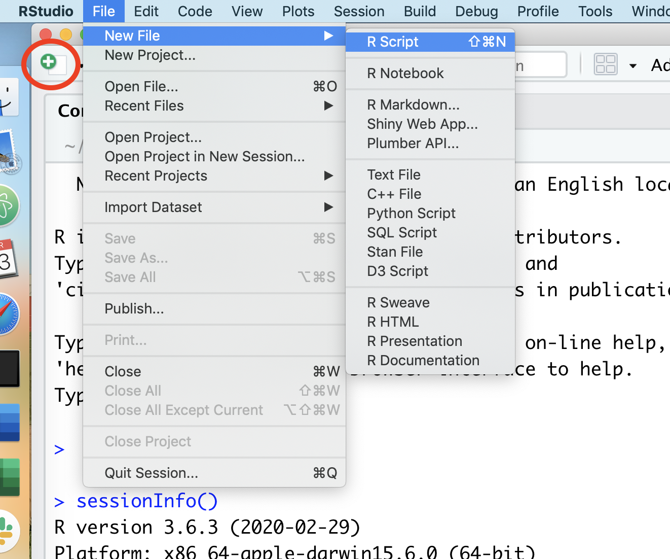
We’ll quickly get to a point where we don’t want to retype multiple lines of code over and over. We can create R scripts that hold lines of code that R Studio will run for us. We can open a new R script by choosing the File menu, then the New File menu, and finally the R Script option. Alternatively, you could click on the icon that contains a white page with a green plus sign on it. I’ve put a red circle around it in the screen shot below
Once you select “R script”, a new panel will open in RStudio.
That upper right panel is where you can type in code. Go ahead and copy and paste the following code into your new R script
library(tidyverse)

r_version <- R.version$version.string

read_csv("https://raw.githubusercontent.com/riffomonas/data/master/comma-survey/comma-survey.csv") %>%
	rename(data=`How would you write the following sentence?`) %>%
	mutate(data=recode(data,
		`Some experts say it's important to drink milk, but the data are inconclusive.` = "Plural",
		`Some experts say it's important to drink milk, but the data is inconclusive.` = "Singular")
	) %>%
	count(data) %>%
	drop_na() %>%
	mutate(percentage = 100 * n/sum(n)) %>%
	ggplot(aes(x=data, y=percentage, fill=data)) +
		geom_col(show.legend=FALSE) +
		labs(x=NULL,
			y="Percentage of respondents",
			title="Is the word 'data' plural or singular?",
			subtitle=r_version) +
		theme_classic()
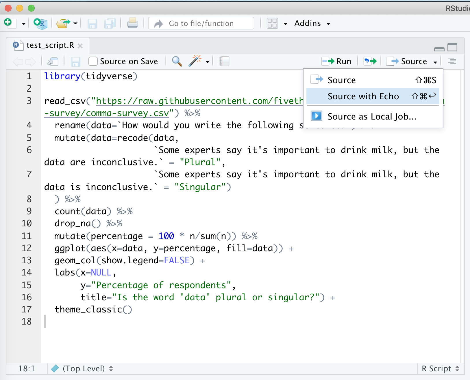
Go ahead and save this as test_script.R. You should have something like this
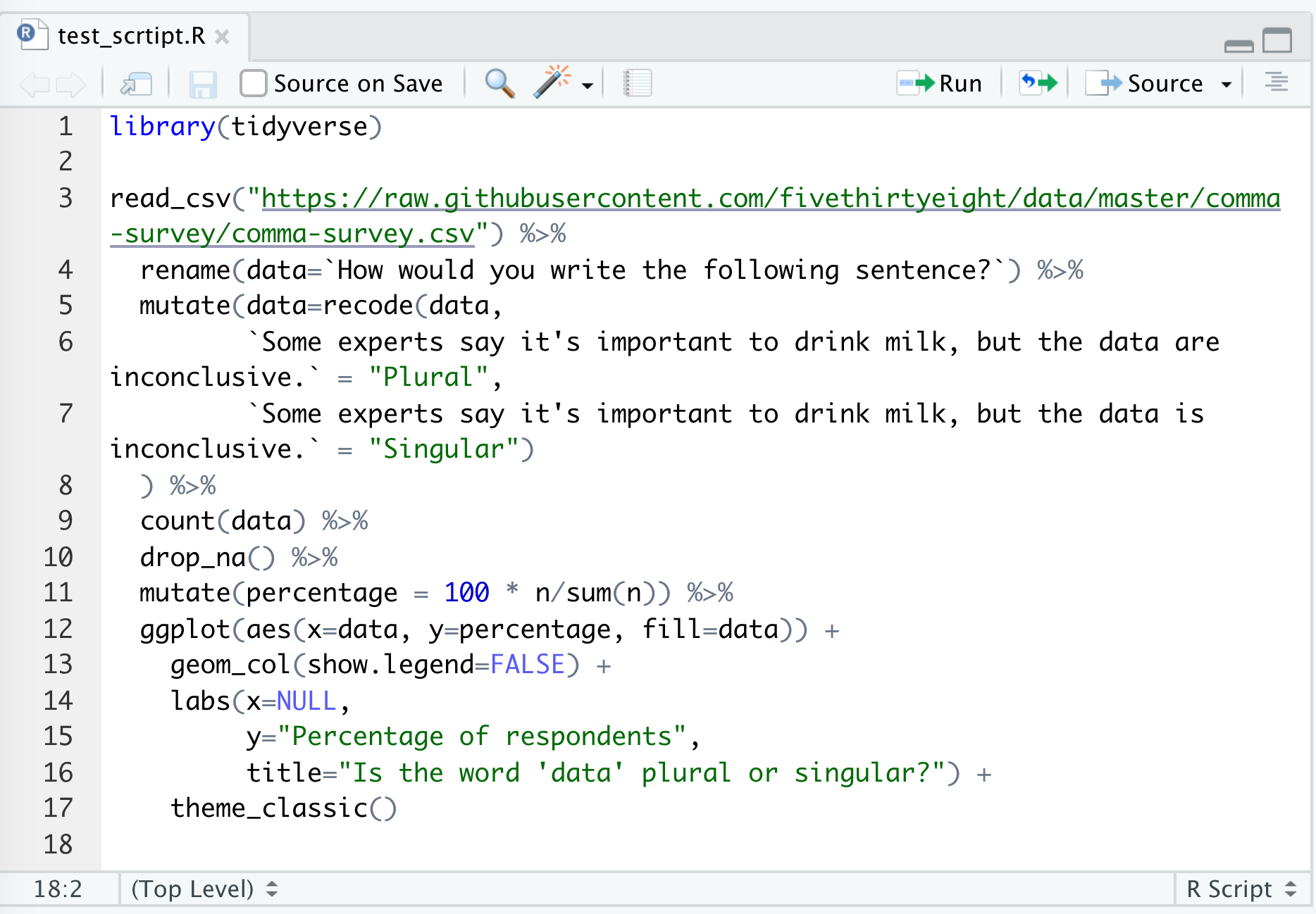
There are several ways to run this script. You could copy and paste all the code to the console window below. An easier way would be to click “Source”, and “Source with Echo”. There are a few other ways to run the code in the script in your console, but this will serve us well for now…
This will run your code in the console window below and will pop out your plot in the lower right corner. Viola! If everything is set up correctly, you should have a plot that looks like mine.
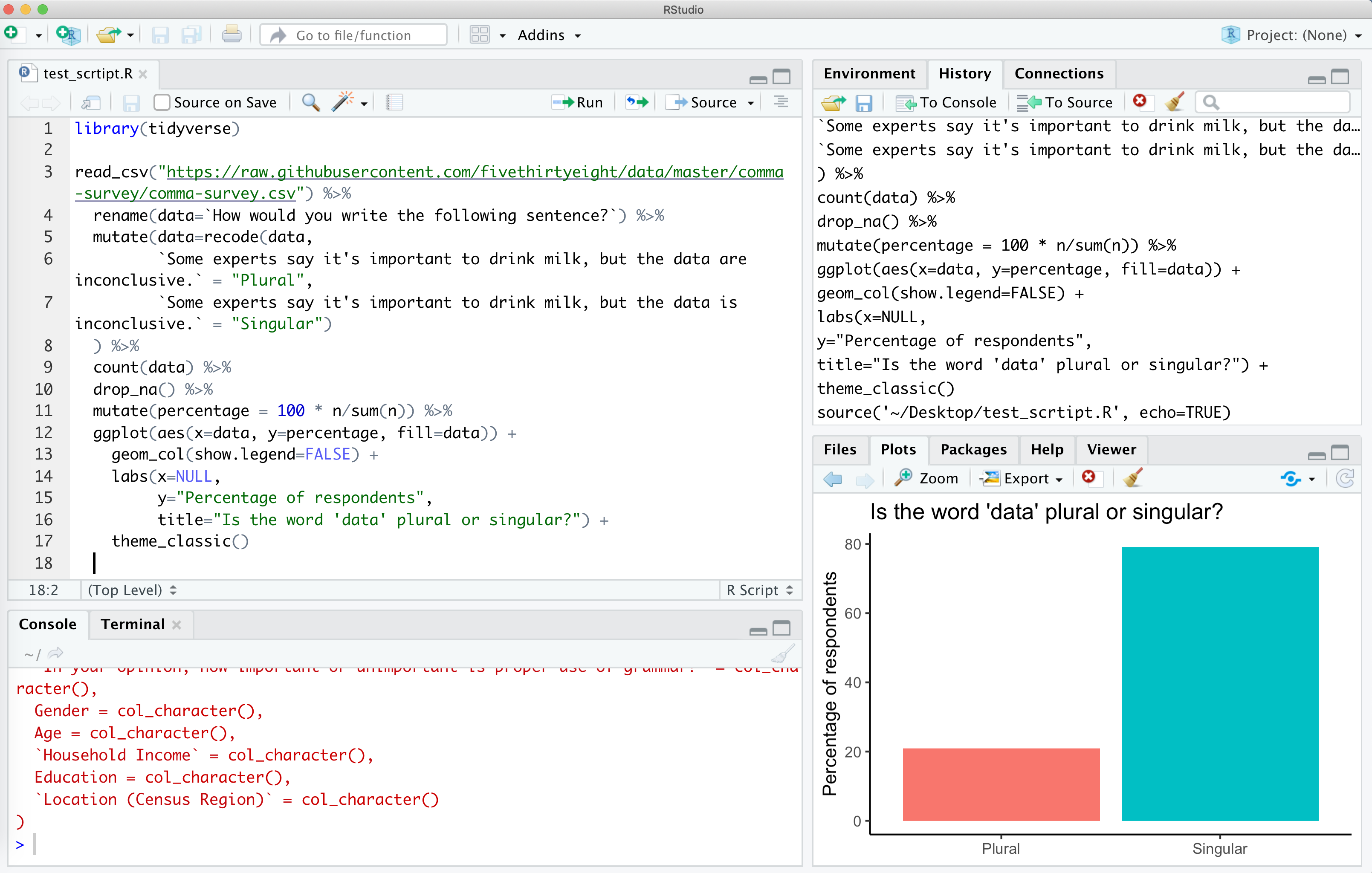
If you don’t get this, make sure you installed the tidyverse package as described above and then make sure you copy and pasted everything from the code block above into a clean R script file.
My setup
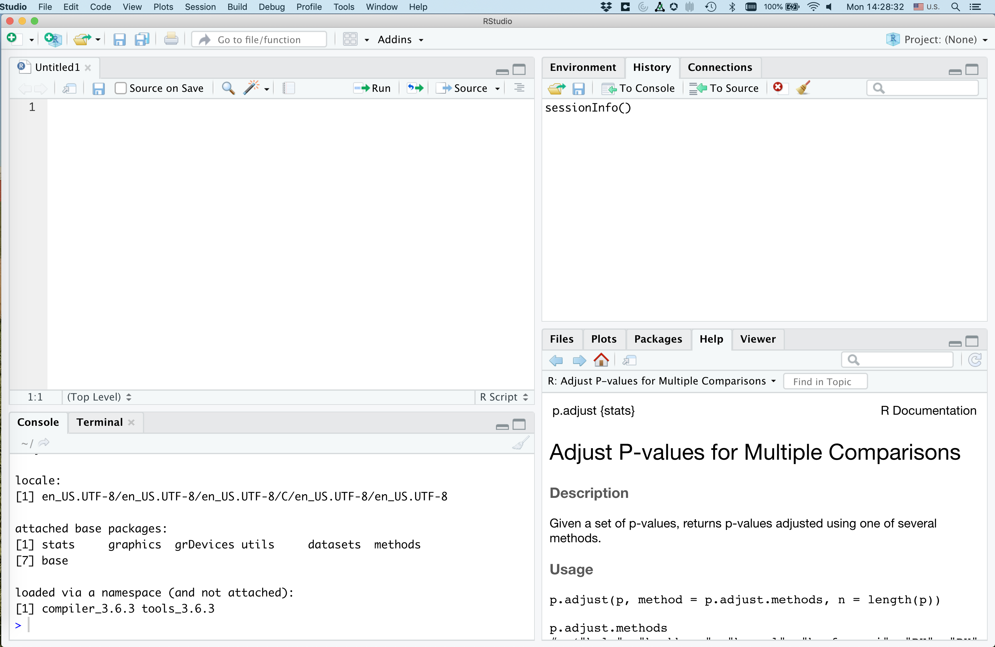
If you run sessionInfo at the console, you will see the version of R and the packages you have installed and attached (more about what this all means later). Here’s what mine looks like.
sessionInfo()
## R version 4.0.3 (2020-10-10)
## Platform: x86_64-apple-darwin17.0 (64-bit)
## Running under: macOS Catalina 10.15.7
##
## Matrix products: default
## BLAS:   /Library/Frameworks/R.framework/Versions/4.0/Resources/lib/libRblas.dylib
## LAPACK: /Library/Frameworks/R.framework/Versions/4.0/Resources/lib/libRlapack.dylib
##
## locale:
## [1] en_US.UTF-8/en_US.UTF-8/en_US.UTF-8/C/en_US.UTF-8/en_US.UTF-8
##
## attached base packages:
## [1] stats     graphics  grDevices utils     datasets  methods   base
##
## other attached packages:
##  [1] forcats_0.5.0   stringr_1.4.0   dplyr_1.0.2     purrr_0.3.4
##  [5] readr_1.4.0     tidyr_1.1.2     tibble_3.0.4    ggplot2_3.3.2
##  [9] tidyverse_1.3.0 knitr_1.30      ezknitr_0.6
##
## loaded via a namespace (and not attached):
##  [1] Rcpp_1.0.5        cellranger_1.1.0  pillar_1.4.6      compiler_4.0.3
##  [5] dbplyr_2.0.0      R.methodsS3_1.8.1 R.utils_2.10.1    tools_4.0.3
##  [9] lubridate_1.7.9.2 jsonlite_1.7.1    evaluate_0.14     lifecycle_0.2.0
## [13] gtable_0.3.0      pkgconfig_2.0.3   rlang_0.4.9       reprex_0.3.0
## [17] cli_2.1.0         rstudioapi_0.13   DBI_1.1.0         haven_2.3.1
## [21] xfun_0.19         withr_2.3.0       xml2_1.3.2        httr_1.4.2
## [25] fs_1.5.0          generics_0.1.0    vctrs_0.3.5       hms_0.5.3
## [29] grid_4.0.3        tidyselect_1.1.0  glue_1.4.2        R6_2.5.0
## [33] fansi_0.4.1       readxl_1.3.1      modelr_0.1.8      magrittr_2.0.1
## [37] ps_1.4.0          backports_1.2.0   scales_1.1.1      ellipsis_0.3.1
## [41] rvest_0.3.6       assertthat_0.2.1  colorspace_2.0-0  stringi_1.5.3
## [45] munsell_0.5.0     broom_0.7.2       crayon_1.3.4      R.oo_1.24.0